(사이킷런) 타이타닉 생존자 예측
Titanic
import numpy as np
import pandas as pd
import matplotlib.pyplot as plt
import seaborn as sns
%matplotlib inline

titanic_df = pd.read_csv('./train.csv')
titanic_df.head(3)
| PassengerId | Survived | Pclass | Name | Sex | Age | SibSp | Parch | Ticket | Fare | Cabin | Embarked | |
|---|---|---|---|---|---|---|---|---|---|---|---|---|
| 0 | 1 | 0 | 3 | Braund, Mr. Owen Harris | male | 22.0 | 1 | 0 | A/5 21171 | 7.2500 | NaN | S |
| 1 | 2 | 1 | 1 | Cumings, Mrs. John Bradley (Florence Briggs Th... | female | 38.0 | 1 | 0 | PC 17599 | 71.2833 | C85 | C |
| 2 | 3 | 1 | 3 | Heikkinen, Miss. Laina | female | 26.0 | 0 | 0 | STON/O2. 3101282 | 7.9250 | NaN | S |
- Passengerid: 탑승자 데이터 일련번호
- survived: 생존 여부, 0 = 사망, 1 = 생존
- Pclass: 티켓의 선실 등급, 1 = 일등석, 2 = 이등석, 3 = 삼등석
- sex: 탑승자 성별
- name: 탑승자 이름
- Age: 탑승자 나이
- sibsp: 같이 탑승한 형제자매 또는 배우자 인원수
- parch: 같이 탑승한 부모님 또는 어린이 인원수
- ticket: 티켓 번호
- fare: 요금
- cabin: 선실 번호
- embarked: 중간 정착 항구 C = Cherbourg, Q = Queenstown, S = Southampton
print(titanic_df.info()) #타이타닉 정보
<class 'pandas.core.frame.DataFrame'>
RangeIndex: 891 entries, 0 to 890
Data columns (total 12 columns):
 #   Column       Non-Null Count  Dtype
---  ------       --------------  -----
 0   PassengerId  891 non-null    int64
 1   Survived     891 non-null    int64
 2   Pclass       891 non-null    int64
 3   Name         891 non-null    object
 4   Sex          891 non-null    object
 5   Age          714 non-null    float64
 6   SibSp        891 non-null    int64
 7   Parch        891 non-null    int64
 8   Ticket       891 non-null    object
 9   Fare         891 non-null    float64
 10  Cabin        204 non-null    object
 11  Embarked     889 non-null    object
dtypes: float64(2), int64(5), object(5)
memory usage: 83.7+ KB
None
#null값 처리
titanic_df['Age'].fillna(titanic_df['Age'].mean(),inplace=True)
titanic_df['Cabin'].fillna('N',inplace=True)
titanic_df['Embarked'].fillna('N',inplace=True)
titanic_df.isnull().sum()
PassengerId    0
Survived       0
Pclass         0
Name           0
Sex            0
Age            0
SibSp          0
Parch          0
Ticket         0
Fare           0
Cabin          0
Embarked       0
dtype: int64
#컬럼 분포
print('Sex 분포: \n',titanic_df['Sex'].value_counts())
print('\n')
print('Cabin 분포: \n',titanic_df['Cabin'].value_counts())
print('\n')
print('Embarked 분포: \n',titanic_df['Embarked'].value_counts())
Sex 분포:
 male      577
female    314
Name: Sex, dtype: int64


Cabin 분포:
 N              687
B96 B98          4
G6               4
C23 C25 C27      4
F33              3
              ...
D21              1
D50              1
A36              1
C30              1
A19              1
Name: Cabin, Length: 148, dtype: int64


Embarked 분포:
 S    644
C    168
Q     77
N      2
Name: Embarked, dtype: int64
#cabin 앞 문자만 추출
titanic_df['Cabin']=titanic_df['Cabin'].str[:1]
print(titanic_df['Cabin'],'\n')
titanic_df['Cabin'].value_counts()
0      N
1      C
2      N
3      C
4      N
      ..
886    N
887    B
888    N
889    C
890    N
Name: Cabin, Length: 891, dtype: object


N    687
C     59
B     47
D     33
E     32
A     15
F     13
G      4
T      1
Name: Cabin, dtype: int64
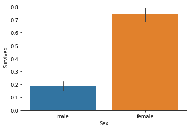
#성별에 따른 생존자
titanic_df.groupby(['Sex','Survived'])['Survived'].count()
Sex     Survived
female  0            81
        1           233
male    0           468
        1           109
Name: Survived, dtype: int64
sns.barplot(x='Sex',y='Survived',data=titanic_df)
<matplotlib.axes._subplots.AxesSubplot at 0x2510af077f0>
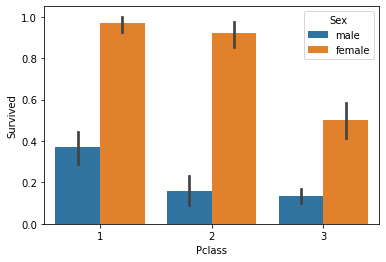
sns.barplot(x='Pclass',y='Survived',hue='Sex',data=titanic_df)
<matplotlib.axes._subplots.AxesSubplot at 0x2511049d2e0>
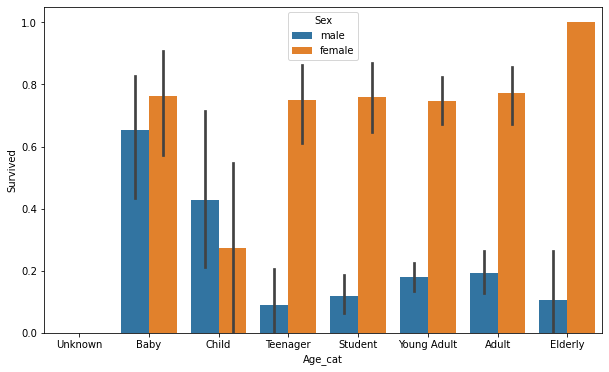
#나이 카테고리 값으로 변경해서 그래프 그리기
# 입력 age에 따라 구분값을 반환하는 함수 설정. DataFrame의 apply lambda식에 사용.
def get_category(age):
    cat = ''
    if age <= -1: cat = 'Unknown'
    elif age <= 5: cat = 'Baby'
    elif age <= 12: cat = 'Child'
    elif age <= 18: cat = 'Teenager'
    elif age <= 25: cat = 'Student'
    elif age <= 35: cat = 'Young Adult'
    elif age <= 60: cat = 'Adult'
    else : cat = 'Elderly'

    return cat

# 막대그래프의 크기 figure를 더 크게 설정
plt.figure(figsize=(10,6))

#X축의 값을 순차적으로 표시하기 위한 설정
group_names = ['Unknown', 'Baby', 'Child', 'Teenager', 'Student', 'Young Adult', 'Adult', 'Elderly']

#위의 함수를 반환값으로(cat 반환)
titanic_df['Age_cat']=titanic_df['Age'].apply(lambda x : get_category(x))
sns.barplot(x='Age_cat',y='Survived',hue='Sex',data=titanic_df,order=group_names)
titanic_df.drop('Age_cat',axis=1,inplace=True)
#인코딩(속성들 숫자형으로)
from sklearn import preprocessing

def encode_features(dataDF):
    features = ['Cabin', 'Sex', 'Embarked']
    for feature in features:
        le = preprocessing.LabelEncoder()
        le = le.fit(dataDF[feature])
        dataDF[feature] = le.transform(dataDF[feature])
    return dataDF

titanic_df=encode_features(titanic_df)
titanic_df
| PassengerId | Survived | Pclass | Name | Sex | Age | SibSp | Parch | Ticket | Fare | Cabin | Embarked | |
|---|---|---|---|---|---|---|---|---|---|---|---|---|
| 0 | 1 | 0 | 3 | Braund, Mr. Owen Harris | 1 | 22.000000 | 1 | 0 | A/5 21171 | 7.2500 | 7 | 3 |
| 1 | 2 | 1 | 1 | Cumings, Mrs. John Bradley (Florence Briggs Th... | 0 | 38.000000 | 1 | 0 | PC 17599 | 71.2833 | 2 | 0 |
| 2 | 3 | 1 | 3 | Heikkinen, Miss. Laina | 0 | 26.000000 | 0 | 0 | STON/O2. 3101282 | 7.9250 | 7 | 3 |
| 3 | 4 | 1 | 1 | Futrelle, Mrs. Jacques Heath (Lily May Peel) | 0 | 35.000000 | 1 | 0 | 113803 | 53.1000 | 2 | 3 |
| 4 | 5 | 0 | 3 | Allen, Mr. William Henry | 1 | 35.000000 | 0 | 0 | 373450 | 8.0500 | 7 | 3 |
| ... | ... | ... | ... | ... | ... | ... | ... | ... | ... | ... | ... | ... |
| 886 | 887 | 0 | 2 | Montvila, Rev. Juozas | 1 | 27.000000 | 0 | 0 | 211536 | 13.0000 | 7 | 3 |
| 887 | 888 | 1 | 1 | Graham, Miss. Margaret Edith | 0 | 19.000000 | 0 | 0 | 112053 | 30.0000 | 1 | 3 |
| 888 | 889 | 0 | 3 | Johnston, Miss. Catherine Helen "Carrie" | 0 | 29.699118 | 1 | 2 | W./C. 6607 | 23.4500 | 7 | 3 |
| 889 | 890 | 1 | 1 | Behr, Mr. Karl Howell | 1 | 26.000000 | 0 | 0 | 111369 | 30.0000 | 2 | 0 |
| 890 | 891 | 0 | 3 | Dooley, Mr. Patrick | 1 | 32.000000 | 0 | 0 | 370376 | 7.7500 | 7 | 2 |
891 rows × 12 columns
#피처 가공 함수 만들기(위에랑 겹침)
from sklearn.preprocessing import LabelEncoder

# Null 처리 함수
def fillna(df):
    df['Age'].fillna(df['Age'].mean(),inplace=True)
    df['Cabin'].fillna('N',inplace=True)
    df['Embarked'].fillna('N',inplace=True)
    df['Fare'].fillna(0,inplace=True)
    return df

# 머신러닝 알고리즘에 불필요한 속성 제거
def drop_features(df):
    df.drop(['PassengerId','Name','Ticket'],axis=1,inplace=True)
    return df

# 레이블 인코딩 수행.
def format_features(df):
    df['Cabin'] = df['Cabin'].str[:1]
    features = ['Cabin','Sex','Embarked']
    for feature in features:
        le = LabelEncoder()
        le = le.fit(df[feature])
        df[feature] = le.transform(df[feature])
    return df

# 앞에서 설정한 Data Preprocessing 함수 호출
def transform_features(df):
    df = fillna(df)
    df = drop_features(df)
    df = format_features(df)
    return df
#재로딩하고 피처,레이블 데이터 세트 추출
titanic_df=pd.read_csv('./train.csv')
y_df=titanic_df['Survived']
X_df=titanic_df.drop('Survived',axis=1)

X_df=transform_features(X_df)
from sklearn.model_selection import train_test_split
X_train,X_test,y_train,y_test=train_test_split(X_df,y_df,test_size=0.2,random_state=11)
#결정트리,랜덤 포레스트,로지스틱 회귀 이용해서 예측
from sklearn.tree import DecisionTreeClassifier
from sklearn.ensemble import RandomForestClassifier
from sklearn.linear_model import LogisticRegression
from sklearn.metrics import accuracy_score

# 결정트리, Random Forest, 로지스틱 회귀를 위한 사이킷런 Classifier 클래스 생성
dt_clf = DecisionTreeClassifier(random_state=11)
rf_clf = RandomForestClassifier(random_state=11)
lr_clf = LogisticRegression()

# DecisionTreeClassifier 학습/예측/평가
dt_clf.fit(X_train , y_train)
dt_pred = dt_clf.predict(X_test)
print('DecisionTreeClassifier 정확도: {0:.4f}'.format(accuracy_score(y_test, dt_pred)))

# RandomForestClassifier 학습/예측/평가
rf_clf.fit(X_train , y_train)
rf_pred = rf_clf.predict(X_test)
print('RandomForestClassifier 정확도:{0:.4f}'.format(accuracy_score(y_test, rf_pred)))

# LogisticRegression 학습/예측/평가
lr_clf.fit(X_train , y_train)
lr_pred = lr_clf.predict(X_test)
print('LogisticRegression 정확도: {0:.4f}'.format(accuracy_score(y_test, lr_pred)))
DecisionTreeClassifier 정확도: 0.7877
RandomForestClassifier 정확도:0.8547
LogisticRegression 정확도: 0.8492


C:\anaconda\lib\site-packages\sklearn\linear_model\_logistic.py:762: ConvergenceWarning: lbfgs failed to converge (status=1):
STOP: TOTAL NO. of ITERATIONS REACHED LIMIT.

Increase the number of iterations (max_iter) or scale the data as shown in:
    https://scikit-learn.org/stable/modules/preprocessing.html
Please also refer to the documentation for alternative solver options:
    https://scikit-learn.org/stable/modules/linear_model.html#logistic-regression
  n_iter_i = _check_optimize_result(
#Kfold 클래스 이용해서 교차 검증 수행
from sklearn.model_selection import KFold

def exec_kfold(clf, folds=5):
    # 폴드 세트를 5개인 KFold객체를 생성, 폴드 수만큼 예측결과 저장을 위한  리스트 객체 생성.
    kfold = KFold(n_splits=folds)
    scores = []

    # KFold 교차 검증 수행.
    for iter_count , (train_index, test_index) in enumerate(kfold.split(X_df)):
        # X_titanic_df 데이터에서 교차 검증별로 학습과 검증 데이터를 가리키는 index 생성
        X_train, X_test = X_df.values[train_index], X_df.values[test_index]
        y_train, y_test = y_df.values[train_index], y_df.values[test_index]

        # Classifier 학습, 예측, 정확도 계산
        clf.fit(X_train, y_train)
        predictions = clf.predict(X_test)
        accuracy = accuracy_score(y_test, predictions)
        scores.append(accuracy)
        print("교차 검증 {0} 정확도: {1:.4f}".format(iter_count, accuracy))

    # 5개 fold에서의 평균 정확도 계산.
    mean_score = np.mean(scores)
    print("평균 정확도: {0:.4f}".format(mean_score))
# exec_kfold 호출
exec_kfold(dt_clf , folds=5)
교차 검증 0 정확도: 0.7542
교차 검증 1 정확도: 0.7809
교차 검증 2 정확도: 0.7865
교차 검증 3 정확도: 0.7697
교차 검증 4 정확도: 0.8202
평균 정확도: 0.7823
#cross_val_score이용해서 검증
from sklearn.model_selection import cross_val_score

scores = cross_val_score(dt_clf, X_df , y_df , cv=5)
for iter_count,accuracy in enumerate(scores):
    print("교차 검증 {0} 정확도: {1:.4f}".format(iter_count, accuracy))

print("평균 정확도: {0:.4f}".format(np.mean(scores)))
교차 검증 0 정확도: 0.7430
교차 검증 1 정확도: 0.7753
교차 검증 2 정확도: 0.7921
교차 검증 3 정확도: 0.7865
교차 검증 4 정확도: 0.8427
평균 정확도: 0.7879
#GridSearchCV 이용해서 검증
from sklearn.model_selection import GridSearchCV

parameters = {'max_depth':[2,3,5,10],
             'min_samples_split':[2,3,5], 'min_samples_leaf':[1,5,8]}

grid_dclf = GridSearchCV(dt_clf , param_grid=parameters , scoring='accuracy' , cv=5)
grid_dclf.fit(X_train , y_train)

print('GridSearchCV 최적 하이퍼 파라미터 :',grid_dclf.best_params_)
print('GridSearchCV 최고 정확도: {0:.4f}'.format(grid_dclf.best_score_))
best_dclf = grid_dclf.best_estimator_

# GridSearchCV의 최적 하이퍼 파라미터로 학습된 Estimator로 예측 및 평가 수행.
dpredictions = best_dclf.predict(X_test)
accuracy = accuracy_score(y_test , dpredictions)
print('테스트 세트에서의 DecisionTreeClassifier 정확도 : {0:.4f}'.format(accuracy))
GridSearchCV 최적 하이퍼 파라미터 : {'max_depth': 3, 'min_samples_leaf': 5, 'min_samples_split': 2}
GridSearchCV 최고 정확도: 0.7992
테스트 세트에서의 DecisionTreeClassifier 정확도 : 0.8715